Explorer3D is oriented towards a multi-scene interactive use. This can be used to follow several goals: first to open several visualization windows simultaneously, and second to observe the behaviour of a set of selected objects in these various windows.
The term view does mainly correspond to the 3d scene window. It also corresponds to less used windows, such as tables or 2D graphs. The user can compute and manipulate several 3D scenes for a unique dataset, mainly to:
Some control have a global effect on 3D scenes; colouring is currently one of them (mainly to identify the of classes in several scenes).
Conversely, many control are not supposed to have a global effect, and rather a local one on a single 3D scene; this stands for clustering, crops, etc.
For this purpose we introduce the notion of active view: the active view is the one that is affected by the execution of a non global control action.
How can we set and highlight the active view?
A view can be set active by giving the focus to its window
Once the view has been set active, the window border gets red (see figure 21).
A view remains active until another one is set active, either explicitely or implicitly.
For instance, computing a new 3D scene makes it active.
Only one view at most is active at any time.
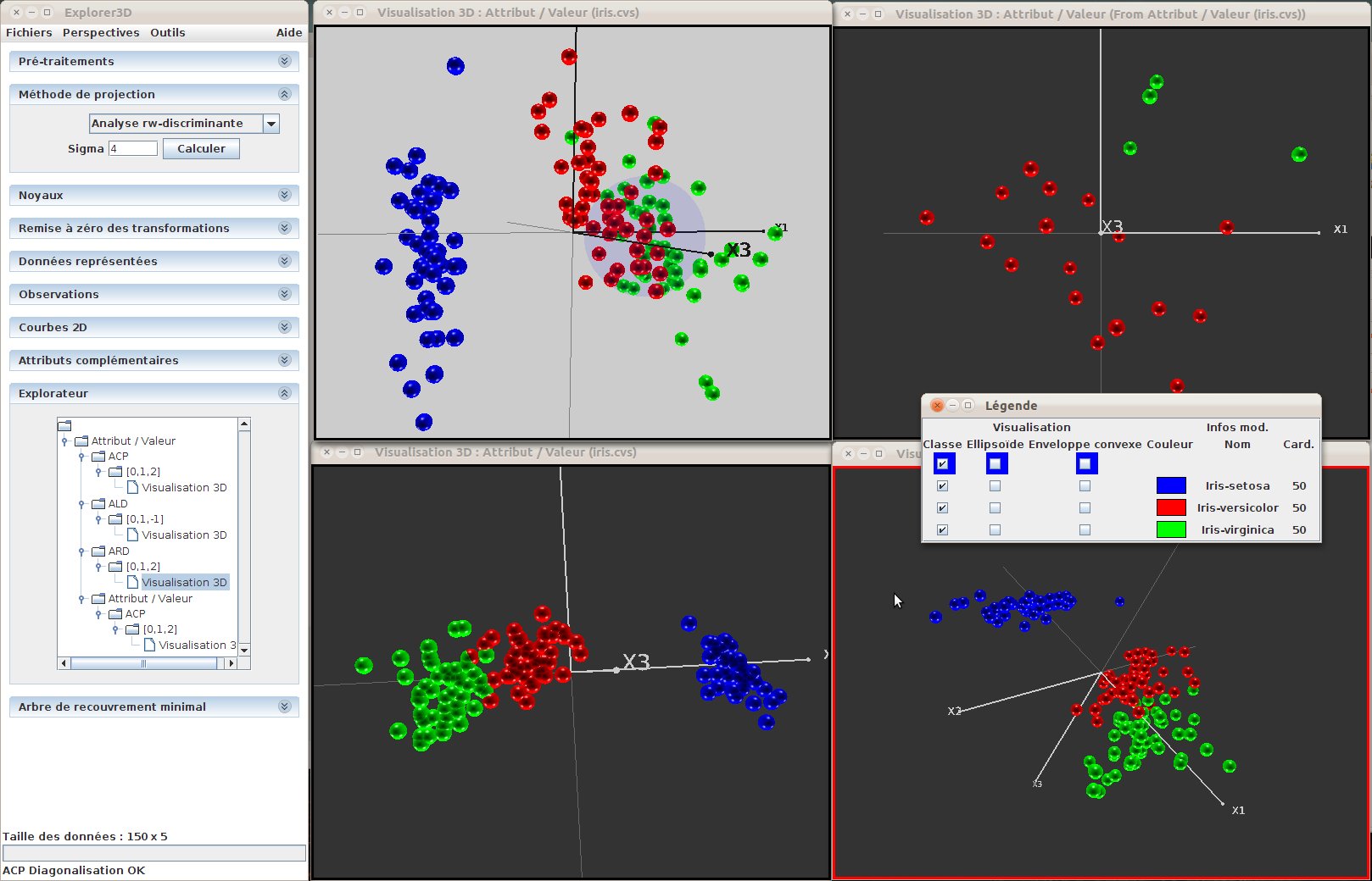
Figure 21: Several simultaneous views. The active view (bottom-right) can be identified by its red border. We can notice that global controls have been used on the views (colouring according to classes), as well as local controls (the lightgrey background of the upper-left scene)
The set of available views can be browsed in the “View Exlorer” sub-window. This sub-window contains a tree-view of the current state of explorer3D, with data input files (data sources) as roots, followed by the projection method, the projection (axes) and finally the view (usually: the 3D scene). The currently active view is highlighted in this browser. Clicking on a given view in the browser gives makes it active.
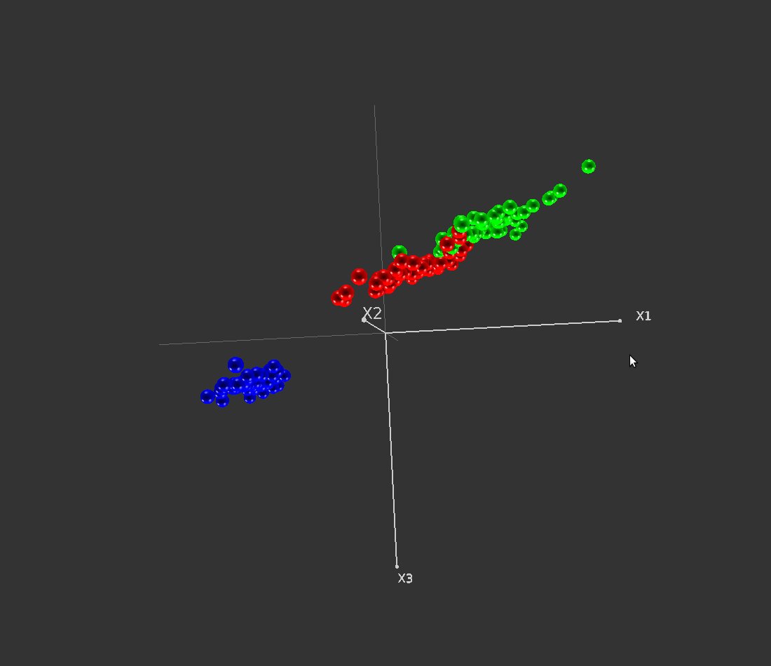
Figure 22 presents the view browser. We can notice that we currently use an “attribute-value” (feature set) data source, on which we computed a PCA and used the 3 main axes of this latter to compute the 3D scene. We can also observe that we used another projection method, were the 3rd projection axis is set to “-1”, which means that the “x3” (z) axis is not used.
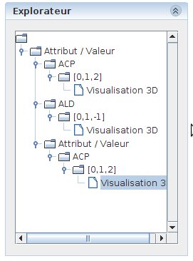
Figure 22: View browser. An “Attribut / Value” (feature set) data source has been used, on which both a PCA and a LDA have been computed. A crop has been computed on one of these views (there is a secondary data source, that is a child of the first one). The crop-based scene is currently active (grey background).
Selected objects are highlighted in the 3D scenes. The set of selected objects is global to all views. This means that selecting an object in one view highlights it in all the views. This can be usefull to look for a given (set of) object(s) throughout several views.
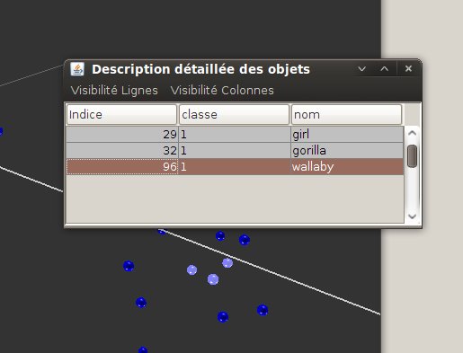
Options allow the user to view a table that contains the additional attributes for the current object set As defined previously, additional attributes consist of data that are not used to compute the object projection, but rather to bring additional knowledge on the objects.
This table contains all of the objects sorted according to their index number. By default, all additional attributes are available. Whether each attribute is displayed can be chosen by the mean of the Column visibility/ additional attributes menu. Projection coordinates can also be displayed using the column visibility / projection coordinates menu. By default, projection coordinates are not displayed.
Object selection is availale in this table, and the set of objects displayed can be limited to the selected ones (see fig. 23). for this purpose, check “Filter (selection)” in the “Lines visibility menu”.
For more details on the selection mechanism, please see section 7.4 .
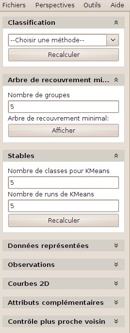
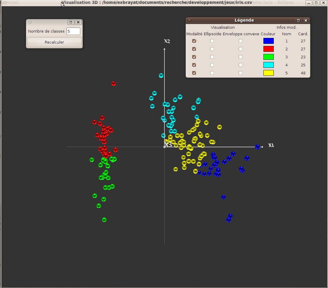
Several clustering methods are available. They can be reached by choosing the “Classification” perspective (see fig.24) in the main window menu. Several of the proposed method shared a common weakness: they are fully stable (they do not always produce exactly the same set of groups). For this reason we encourage the user to compute them several times (using the “recompute” button) to ensure a good understanding of the methods stability w.r.t. the current dataset (let us also underline that the “Recompute” button should also be pressed if the classification parameters, if any, such as the number of groups to produce, have been modified).
when opening
once a method has been chosen
Figure 24: “classification” perspective
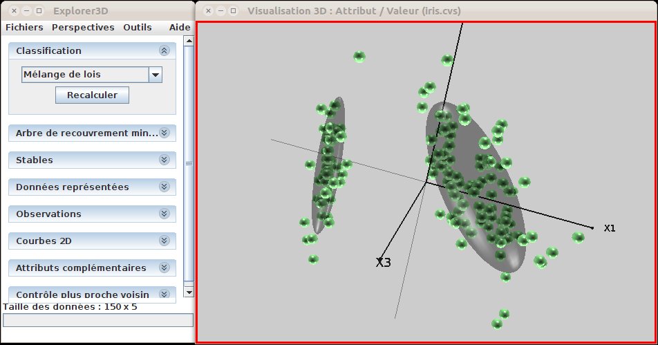
Gaussian mixture classification is built on the idea that objects are distributed according to a ste of multivariate gaussian laws. A technique is thus use to compute the most likely set of underlying laws. Each computed law is displayed by the mean of an ellipsoid that is centered oriented and sized as the law (see fig. 25). The current method (which relies on the klustakwik algorithm) does automatically compute the number of laws.
The principle under that very standard hard clustering method, consists in producing clusters of similar diameters. To be more precise, this algorithm minimizes the sum of the distance of each object to the nearest cluster center. The user first sets the expected number of groups. Group Centers are then randomly initialized and each object is put in to the group of the nearest center. Each center is then updated to the barycenter of the group objects. This process is iterated until stabilization (or a maximum number of iterations is reached). In our current implementation, the default number of centers is set to 5. The user can modify this number and recompute the corresponding clustering result.
Kmeans being not stable, an additional tool is proposed, that computes the stable components. This tool is accessible through the “stables” subwindow. a stable is a set of object that are “always” put in the same cluster by a given clustering method (i.e. kmeans in our software). By “always” we mean in any of a given number of runs of the clustering method. In this tool we can choose the number of classes and also the number of runs to be conducted. Once the runs have all been done, the resulting set of stables is displayed. Stables are currently computed for kmeans only.
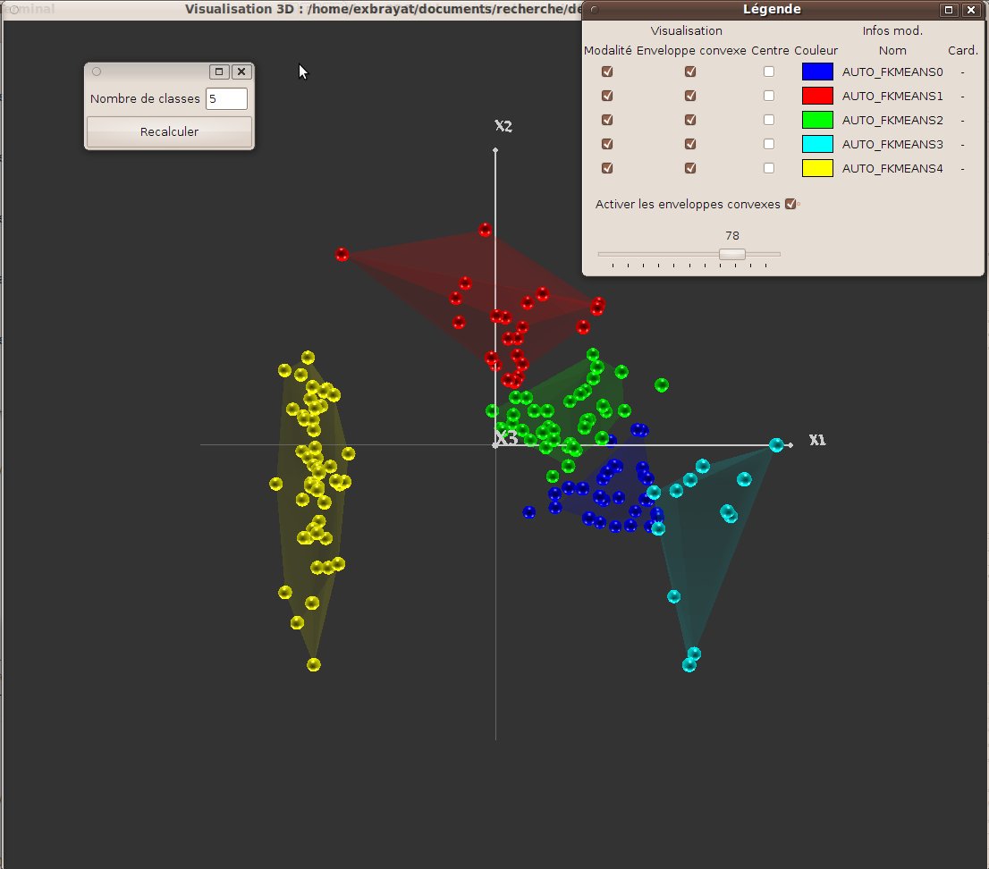
This method is derived from the former one, where each object now belongs to all of the groups at a certain level (degree). The degree is related to the distanceto the center. The sum of degrees is equal to 1. Here again the user can choose the number of centers (default: 5). On one hand, the interest behind this method is to leave more freedom of interpretation to the user. On the other hand, visualization is bit more tricky. We thus developed a specific technic, based on convex envelops, that we did already partly present in section 7.8. Two kinds of information has to be displayed : first, the main group of an object, and second the set of objects that belong to a group “to a given degree”. The main class is displayed using a classical legend. Concerning the “degree”, we use convex envelops (see fig. 27): for each group (or a set of groups) we display the set of objects that belong to it “to a certain degree”, i.e. for which the degree of belonging is “higher that x percent” (remind that we assume that the sum of degrees is 1). The current value of the x threshold can be set using a slider, and the evolution of envelops can thus be observed dynamically. One can notice that this tool can also be used when a fuzzy classification is given as an input and thus coming from a third-tier tool.
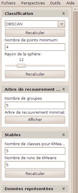
Differing from the former methods, that rely on the distance to a given group center, and thus lead to spherically-structured groups, density-based methods build groups starting from the dense parts of the objects space. Objects are then aggregated in groups depending on their neighboorhood (diffusion). Such methods are relevant when objects are structured in dense, arbitrary shaped groups.
Two parameters can be manually set: first the neighborhood radius (the maximum distance within which two objects are considered as neighbors), and the minimum group cardinality (how many neighbors are needed at least to form a group). In order to help the user to set the radius, a sphere is displayed at the enter of the 3D scene.
Figure 28 presents the result of a DBSCAN clustering. We can notice that the first group consists of the isolated objects (i.e. the ones that do not belong to a cluster). This group might be empty.
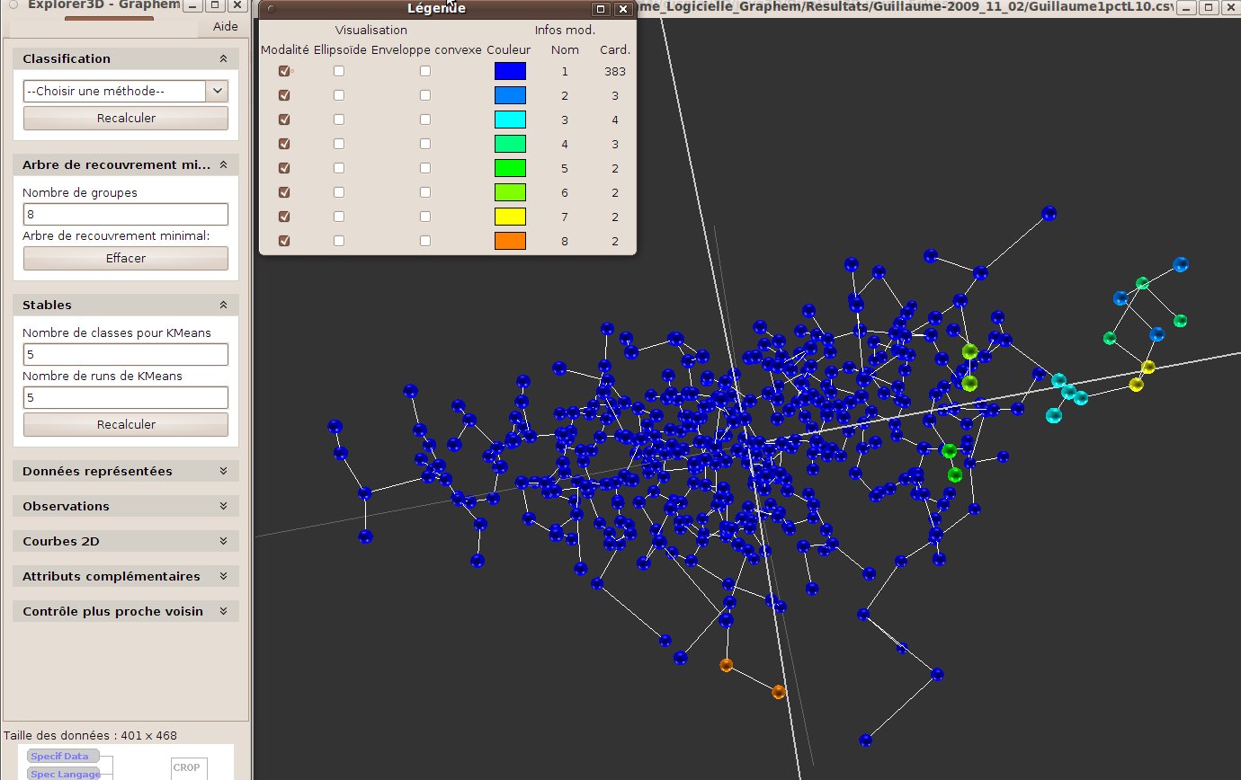
The minimum spanning tree is a tree that links the objects displayed. Briefly speaking, this tree links each object to its nearest neighbor, starting from the nearest pair of objects). Visualising this tree shows how objects are linked from near to near. A long link will highlight the existence of two distant groups, etc.
A hierarchical classification consists in grouping objects starting from the nearest ones, always adding the nearest remaining one, which might be either a object or an already formed group. There exists several ways to compute the distance between two groups. The one we use is called “minimal jump”: The distance between an object and a group is the distance between the object and the object opf the group that is the nearest to him. Between two groups, it is the minimum distance between two objects that belong to each of the group respectively. We produce a classification tree, called dendrogram. Dendrograms are very common, for instance to classify species. While they are usually display in a flat manner, we propose to view them directly in the 3D scene (see fig. 29).
The reader might notice the strong link between the minimum spanning tree and the hierarchical classification based on minimal jump. The number of clusters to be formed is set by the user. Forming the groups does simply correspond to cut the tree at a certain level, starting from the root, where the number of branches equals the expected number of groups.
This tool is an experimental one the user is encouraged to test. This tool can be reached through the “Tools/Interaction” menu. It allows to set a list of relative distance constraints, in order to ask for objects to be moved closer or far away, and to modify the projection dimensions in order to respect these constraints as much as possible while introducing as few global distorsion as possible. We firts invite the user to try the “Comparison” tool.
Several constraints should be entered and taken into account for a space modification.
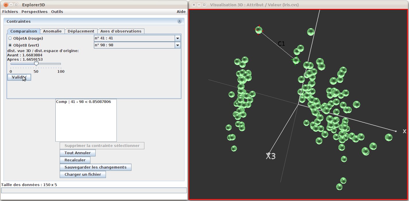
Figure 30: Distance constraints: The two objects concerned can be identified in the 3D scene (object A-41 :red target; object B-98 : green target). The constraint asks for the two objects to be moved closer (slider in the left-most window, and the constraint is textually displayed in the bottom-left list (Comp | 41-98 < 0.85...)
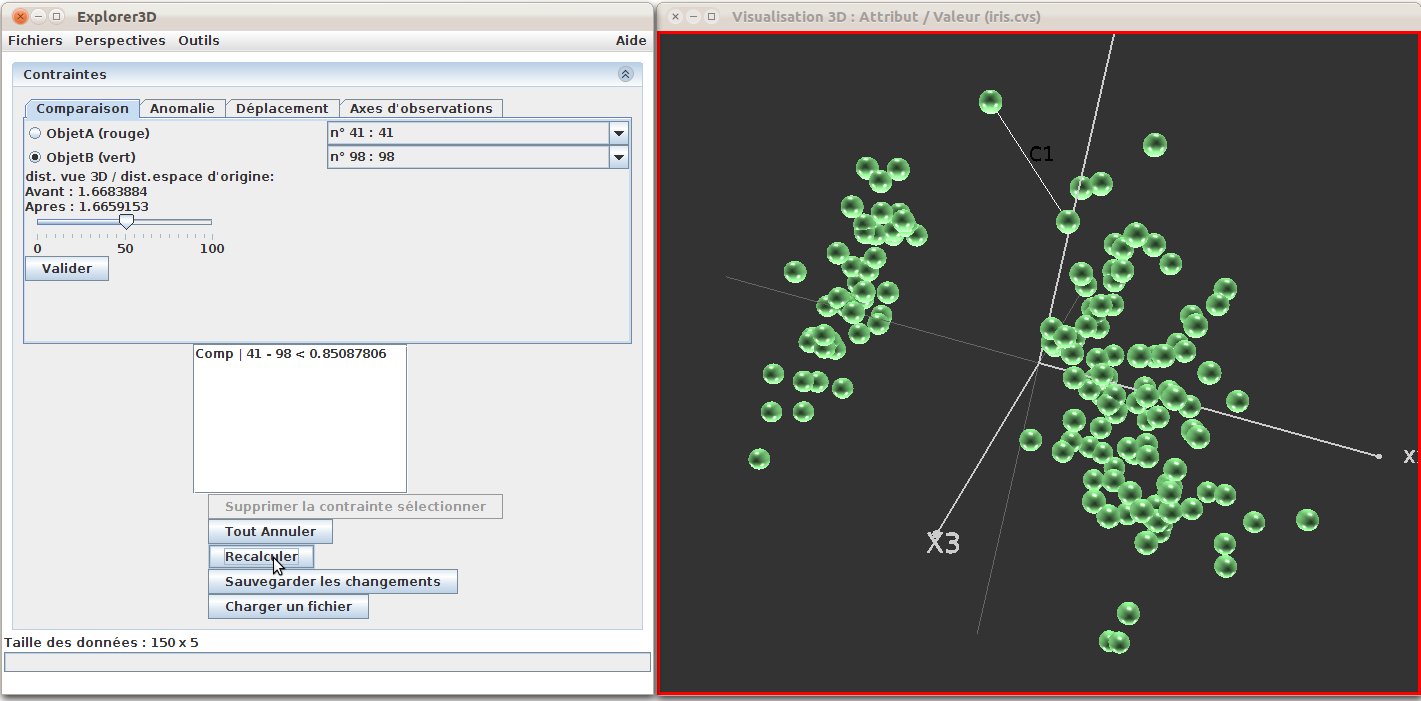
Figure 31: Distance constraints: the constraint has been integrated in the projection framework. We can see that projection has been modified and that the two objects are now closer.
The Anomaly tool allow the user to modify the relative positionning of three objects. We thus manipulate three objects A, B and C. The underlying idea consists in modifying distance A-C with regards to distance A-B. In other words, the user expect C to be moved close to or away from A so that in becomes closer or more far away from A than B.
We proceed as before, using the checkboxes and the scene to set A, B and C and then modifying the distance rate using the slider.
The underlying idea consists in changing the neighborhood of an object. This is a rather complex method the user might use with care. The user must first set the target neighborhood by selecting the objects that belong to it, and then by clicking on “Add”. She must then click on “object to move”, and click on the corresponding object. Just like before, the user than has to click on “OK” and then on “Run !”.
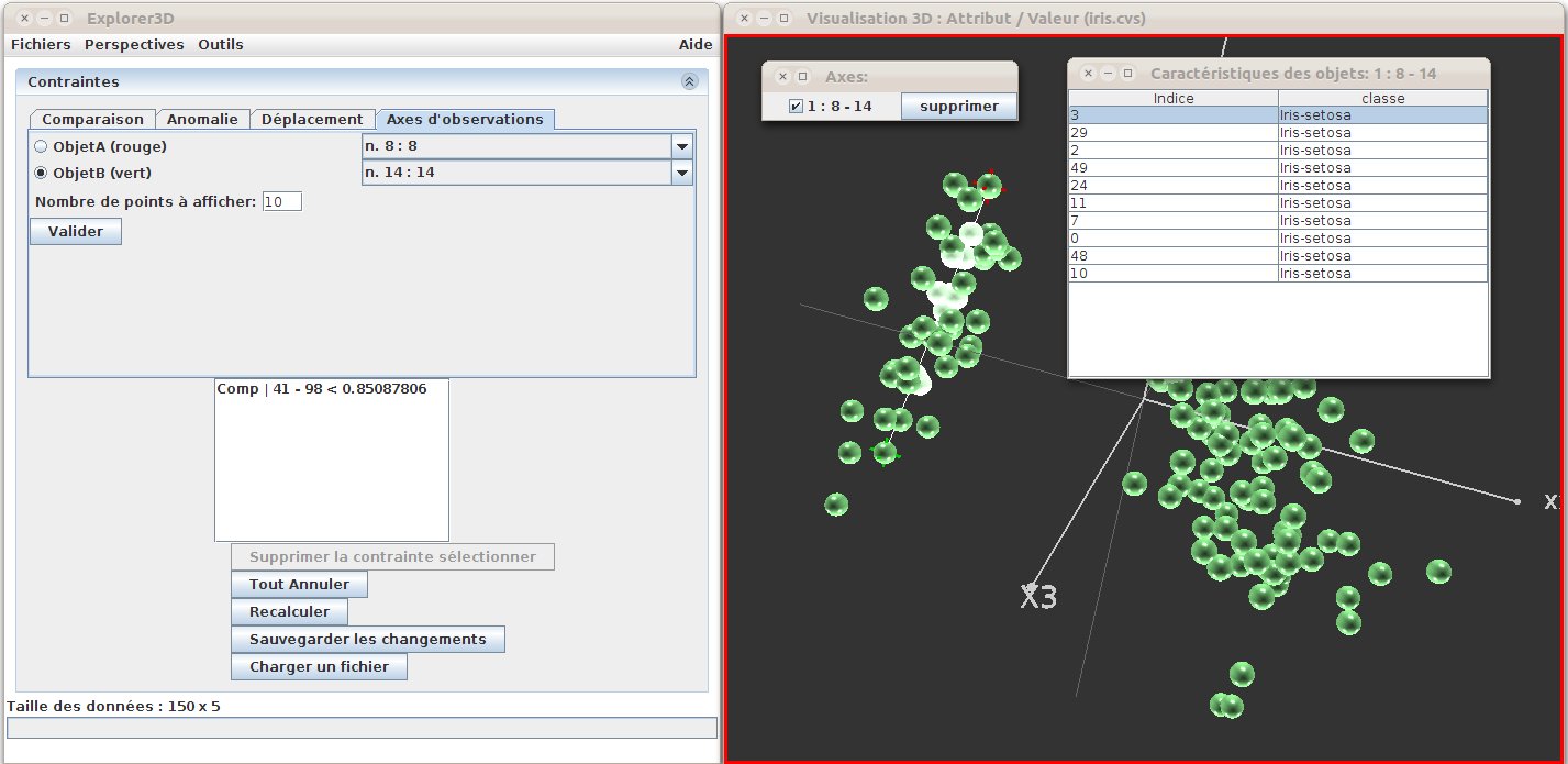
In order to observe a subset of objects along a given axis, the user can set observations axes. For this purpose, the user chooses the “Observation Axis” tab (fig. 32), and then chooses to objects to from the ends of the axis (by clicking on them in the 3D scene). The number of objects to be displayed is then set (default: 10), and the user clicks on “OK”. The 10 objects that are the nearest ones to the segment are then selected, and a table containing informatin about these objects (global rank and additional attributes) is then displayed (“Objects description” window). Several axes can be available simultaneously. The user selects the ones to be displayed / hidden using the “Axis:” window.
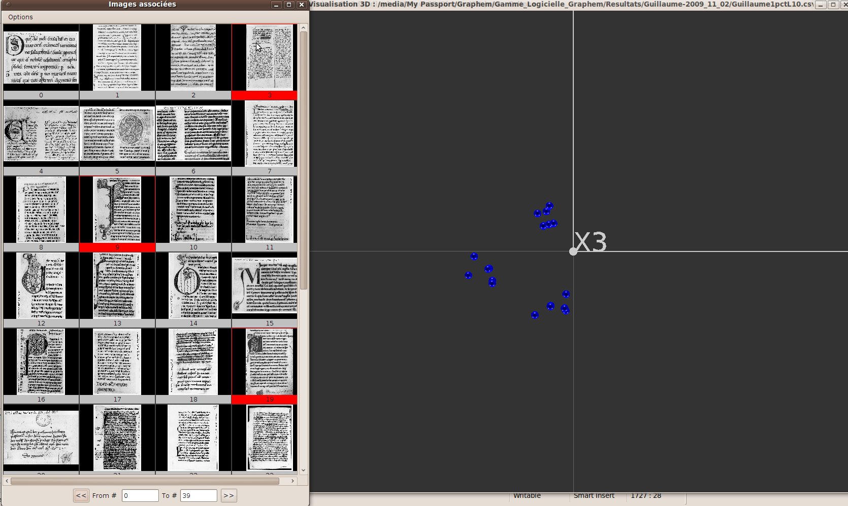
In order to make the projection space more readable, we add the possibility to only display a subset of the objects, based on the associated pictures. For this tool to work properly, the “associated data” additional attribute must have been set. The user then activates the tool by checking “Explore from Images” in the “Tools” menu. All objects are then removed (hidden) from the 3D scene and a new window, “Associated pictures” opens, where the user can choose the objects he wants to display (fig. 33). The user then chooses the pictures he wants to observe, either in the drop-down list available at the top of the window (“List” tab + validate) or by typing the picture file name (“Name” tab + validate). Each time a new picture is choosen, this picture gets displayed in the window, and the corresponding objects is set visible back in the 3D scene. When a picture gets clicked, the object is swaped to the “selected” state, and the corresponding shape in the 3D scene becomes haighlighted. Clicking again on a picture causes the object to be deselected.
The object “n” neighbors can be displayed, together with their picture. the value of “n” is set by the user in the “Neighbors” tab, and is by default set to 0. When an object gets hidden back, so are its neighbors.
This explroation can be superimposed with the standard dynamic display of pictures in the 3D scene.
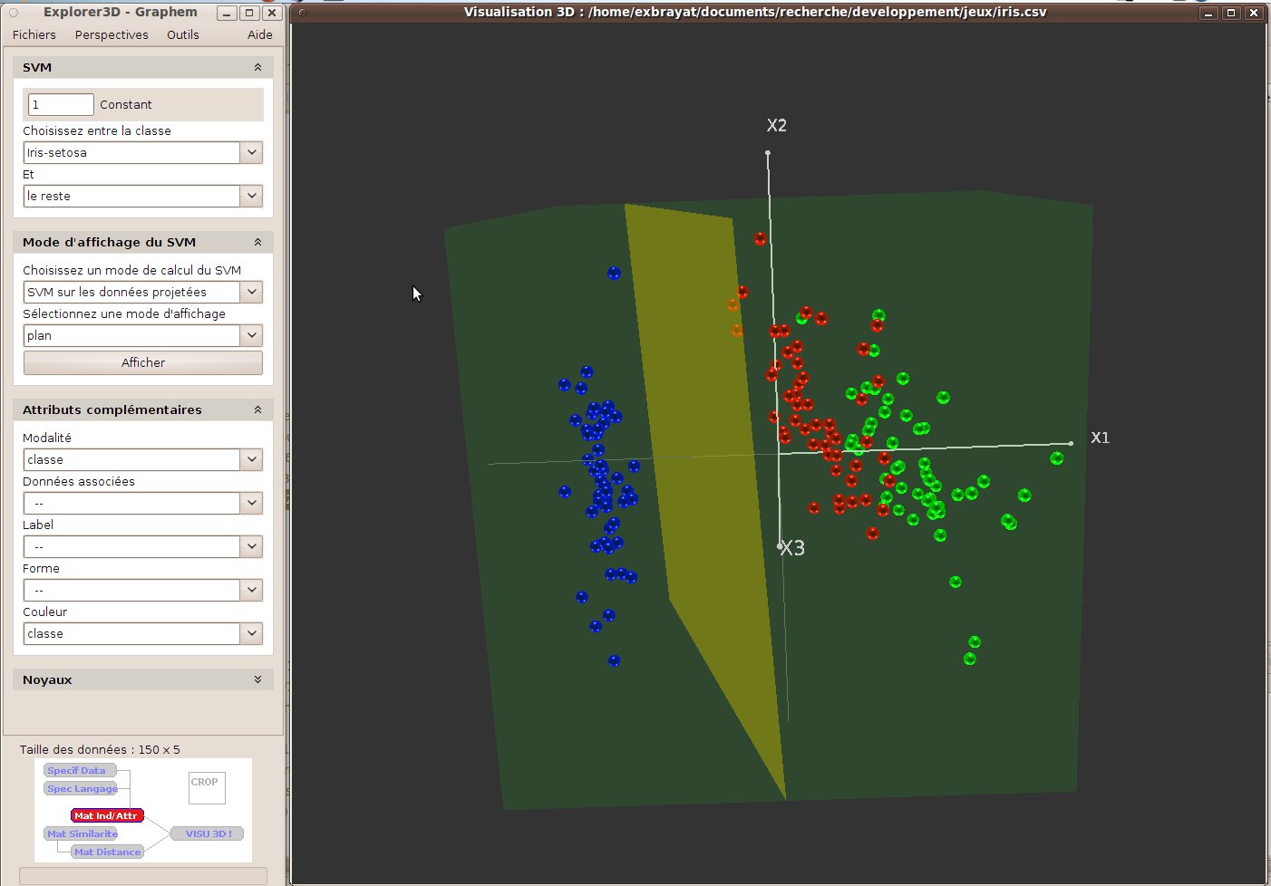
SVM stands for support vector machine, which are a classification tool that try to separate two groups of objects using a (hyper)plane. They are thus usable when the user knows the class of at least a subset of the objects.
In the easiest configuration, the separation is a plane in the original or projection space, that perfectly separates the groups. Moreover, this plane must be as far as possible of the two groups (i.e. as central as possible). Such a clear separation is not always available. Either the groups might be somehow mixed, or separated by a surface that does not look like a plane. For this reason, SVM are usually used together with kernels (see section 8.7).
If more that two groups exist, it is possible either to define a SVM between two of the groups or between one group and all the remaining ones.
In Explorer3D the SVM control are accessed through the SVM perspective. The class attribute must have been set before using SVMs.
Figure 34 illustrates a SVM simple case, based on the very standard “iris” dataset. We can see that a plane has been drawn in the 3D scence that materializes a SVM computed between the “iris-setosa” group on one side, and the remaining groups on the other side.
Availables commands are as follows:
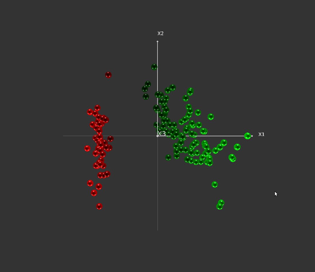
The colouring mode uses a colour grade to recolor the objects relatively to their side and distance to the hyperplane (red on one side, green on the other one). Figure 35 illustrates this mode.
the “replace 3rd axis” used the x3 projection axis to materialize the side and distance to the hyperplane for each object. Projection based on input features is then limited to the “x1” and “x2” axes. Figure 36 illustrates this mode.
Theses two modes can be used with both SVM computed in the original or projected space.
Kernels are powerful tools that have been widely used in machin learning due originally to SVM. As we said before, identified an separating hyperplane is not always easy nor feasible both in the original and projected space. Kernels “compute” new attributes based on some combinations of the original ones. Most of these combinations are not linear, but must anyway respect some criterias. The “trick” with kernels is that in fact they all allow to compute a distance between object without really computing the new attributes, and thus propose various and potentially complex spaces at a low cost. We invite the reader to consult the abundant bibliography of the field for more details.
In Explorer3D kernels are available in the “SVM” and “ND->3D” perspectives. The “Kernels” subwindow allow the user to select a given kernel in a drop-down list and to set the potential parameters of that kernel. Once a kernel has been choosen , it is applied on any new peojection (click on the “Compute” button of the “Projection Methode” subwindow to apply the kernel to the current scene).
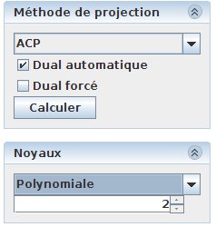
Figure 37: kernel control subwindow. We can see that a polynomial kernel has been choosen, with a degree 2 polynom.
We just list the kernels available in Explorer3D and encourage the reader to refer to kernels litterature to get more details:
Even not kowing much on their specificities, the newby user might test them, looking for an interesting projection space.
The “2D Curves” subwindow allow the user to use various additional curves:
This tool allow the user to connect a third-tier software to Explorer3D , in order to visualize objects and additional data coming from this third-tier software. This function gets activated through the option window (see section 7.7). Explorer3D then listens on a given port (currently port 50 000), and waits for text commands sent using the json format.
The list of commands available is quite simple for the moment, and focus on receiving a set of objects features et on setting or updating their class (and, by the way, their colouring)
``msg'':''set-data''), then the objects description ("val" : [ [object1], [object2], ...]). Here is an example with 4 objects described by four features:
{
  "val": [
    [
      0.09995818,
      0.8450656,
      0.31611204,
      0.9885413
    ],
    [
      0.20870173,
      0.6817836,
      0.30197513,
      0.20966005
    ],
    [
      0.95933825,
      0.7643002,
      0.23336774,
      0.7409621
    ],
    [
      0.075930595,
      0.12991834,
      0.6995411,
      0.092056274
    ]
  ],
  "msg": "set-data"
}
``msg'':''set-classes''), then the number of classes (``nbclasses'': value) and last the class value for each object, sorted in the same order as objects in the “set-data” message ("val" : [ [classe_object1], [classe_object2], ...]).
Here is an example with our set of 4 objects: there are 2 classes; the 3 first objects belong to class 1, the fourth one belongs to class 0 :
{
  "val": [
    1,
    1,
    1,
    0
  ],
  "msg": "set-classes",
  "nbclasses": 2
}
``msg'':''set-classes-fast'') and the list of changes. This latter consists of a table ("val" : [ [classe_object1], [classe_object2], [jump_objects], ...]), the encoding of which is as follows: values ar sorted as the objects appeared in the “set-data” command. A positive value stands for a new class value of the corresponding object; a negative value indicates a jump in the set (objects the class of which is not modified). Here is an example with our 4 objects; The class of the two first objects is not modified (jump 2). The class of the third one is set to 0. The class of the fourth one is not modified (jump 1).
{
  "val": [
    -2,
    0,
    -1
  ],
  "msg": "set-classes-fast"
}
The data import tool is open when the user tries to laod a file with an unknown format.
It might also be directly open to format an input file, through the “Files / Data import tool” menu.
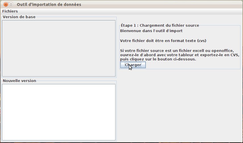
This rather intuitive tool does first load the source file (fig. 38).
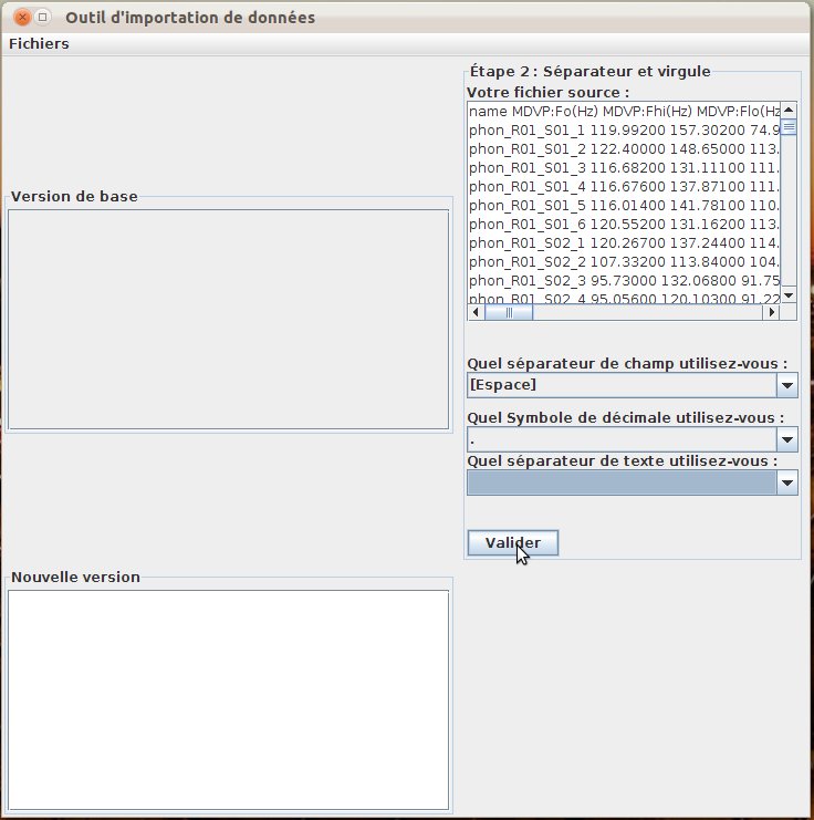
The user then indicates the delimiters used in the file: field separator, dot symbol and text separator (fig. 39). A view of the input file is available during this step.
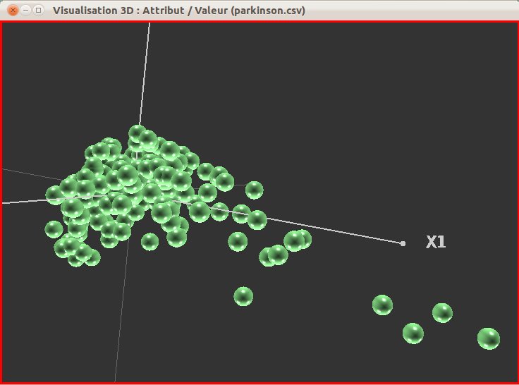
In the proposed example we use the “Parkinson” dataset (UC Irvine machine learning repository).
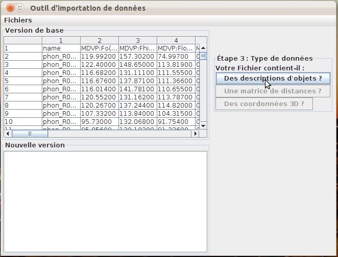
During the next step, the source file is cut according to the delimiters and presented as a table (fig. 40); the user indicates the kind of data that is stored in this file.
In the current implementation, only feature sets files are managed by the import tool.
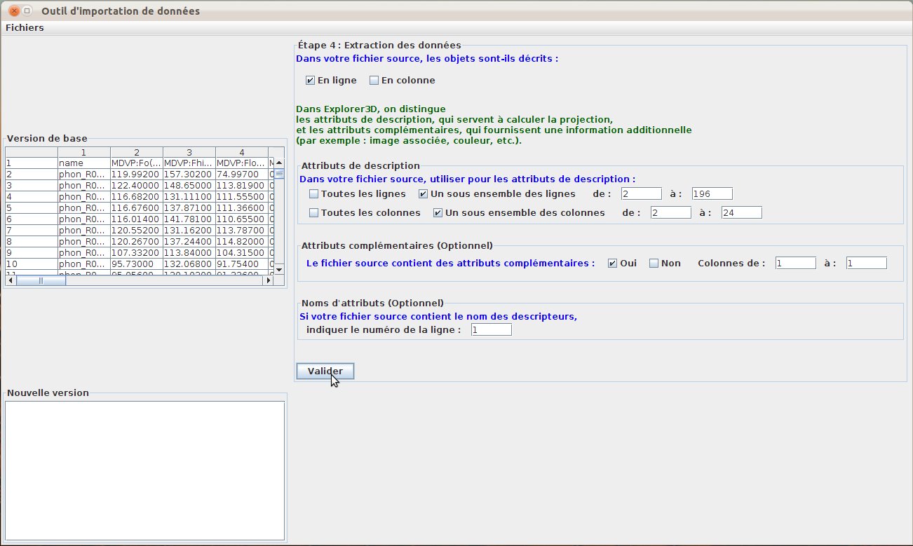
The user then indicates whether the features of an object are organized as a row or as a column (fig. 41).
In our example file, a row correspond to the description of an object, and the projection-relevant features are stored in rows 2 to 196 and in columns 2 to 24.
The first column contains the object names (this is an additional attribute).
The first row contains the names of attributes.
In the current release, description features and additional attributes might not be interlaced (i.e. there is exactly one block of features and at most one block of additional attributes).
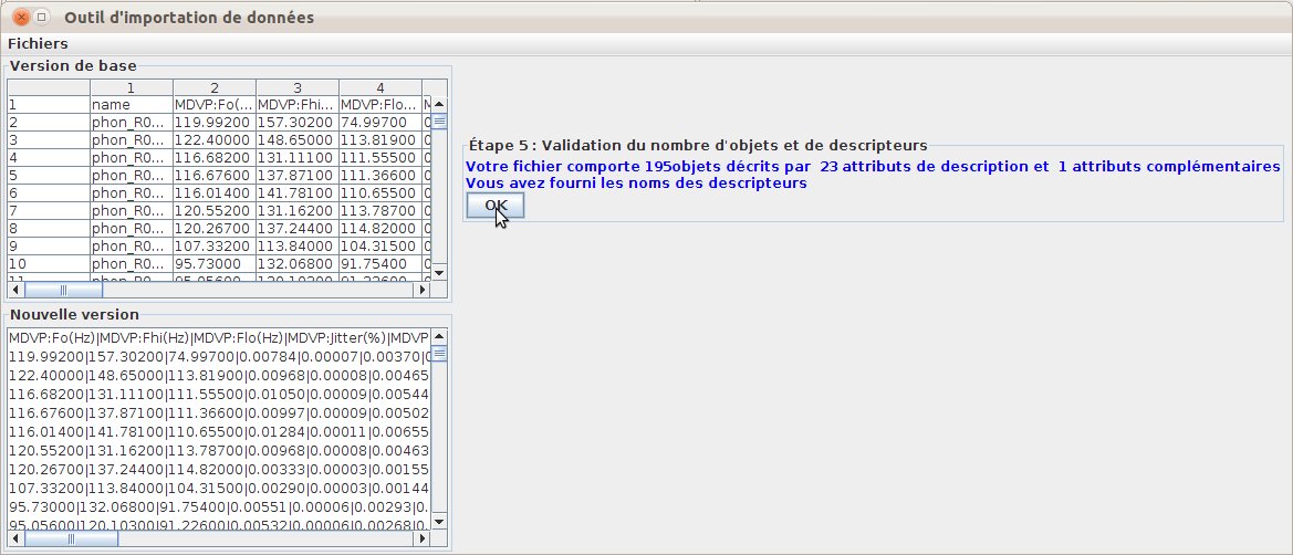
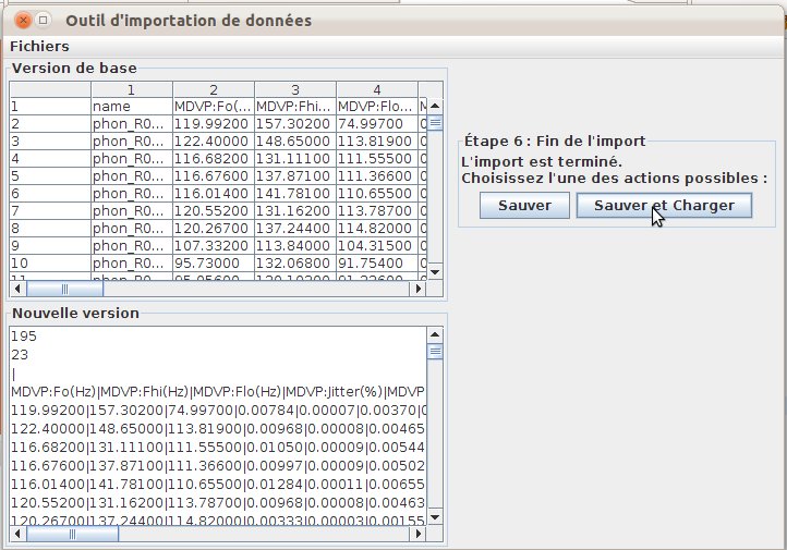
The import then proposes a summary of the imported data (fig. 42), then a view of the final imported file using the Explorer3D format (fig. 43). The user can then either save the file or save it and compute a projection. Figure 44 presents the PCA computed after importing the Parkinson dataset.