Several techniques are currently proposed in the “Projection Method” sub-window (reached through the “Perspectives / ND -> 3D” menu). The actual method is chosen from a list. Currently available methods are:
The “Projection Method” sub-window is tightly associated with the “Pre-treatment” sub-window. This latter is used to apply to data a so-called conditioning. This window offers various treatments to be done on data before applying the projection method.
A check-box allows to choose wether data has to be centered or not. Centering means that the values of each feature are translated so that their is zero. This pre-treatment has to be done for ACP, and might be suitable for other method.
The data variance can be modified depending on the value chosen on the “Reduction method” list: with Raw data variance is not modified; with Reduced variables values are rescaled so that the variance gets equal to 1 –this option is suitable for PCA–; with Normalized distances the values are rescaled so that the amplitude gets equal to 2, and thus, together with data centering, values are between -1 and +1.
We currently propose a single projection method, which consists in a linear multidimensional scaling (MDS), that is a linear projection that computes 3D coordinates so that the distances between pairs of projected objects do correspond as much to their distances in the matrix. Theoretically speaking, this projection stands if the input matrix does really contain distances (with triangular inequality), in which case we can consider that these distances were computed in a high-dimension space, and we thus make some kind of dimensionality reducation. No pre-treatment is available.
We did recently had kernel methods. Those are presented in a specific section (8.7). Kernel methods can be found in the “kernel” sub-window. They allow for the computation of non euclidean distances. For instance, using the “isomap” kernal, we will obtain a new projection, were the only original distances that are kept in the projection space are the ones between nearby objects (this kind of kernel is usually suited when the user knows or guesses that objects are placed on the surface of some non plane surface (i.e. a mathematical variety).
In the case of 3D coordinates, projection is identical to input data. Centering and dimension dilatation are available (see section 7.4).
Additional attributes are given as input but not directly used in the object spatial projection. They can for instance consist of the class of the object, an associated image file name, etc. Five kinds of display modes are currently available:
When identifying groups of objects, the user can either associate a single group to each object, or choose a fuzzy classification, where each object belongs to each group to a certain level. While standard classification relies on a single attribute, multiclassification relies on several numerical attributes, each one corresponding to the level of belonging to a given class. In Explorer3D for a given object, the sum of these levels must be equals to 1.
Multiclassification can be visualized as follows: In the “classes” dropbox, the user chooses the special value “–Multiclasses–”. A secondary list is then displayed in which the user has to select the list of class attributes. The resulting display mode is similar to the one describe in the fuzzy kmean-method (see section 8.3.3).
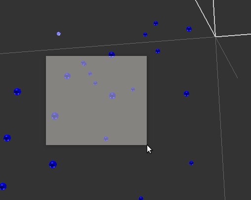
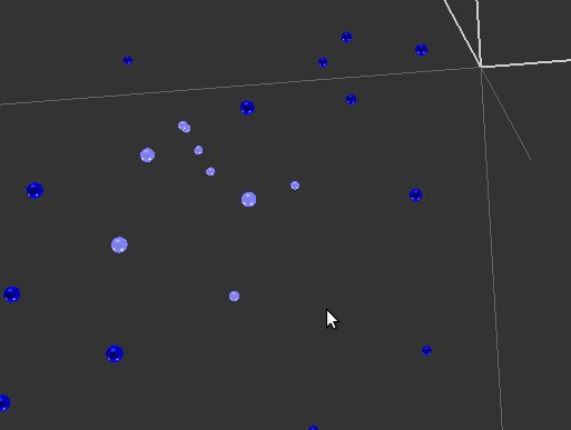
If an “associated data” attribute has been defined, then the image corresponding to each object can be displayed on the basis of the file name stored in this attribute. Image display can be either static or dynamic. Dynamic display occurs when the mouse pointer passes over a given object. The corresponding image is then displayed, and hidden back when the mouse pointer leaves the object. Dynamic display of images is optionanl and occurs only if “Show pictures when mouse is over” is checked. Static image display is controled through the popup menu that opens when the user makes a right-clic –on a given object– with her mouse (see section 7.3.3).
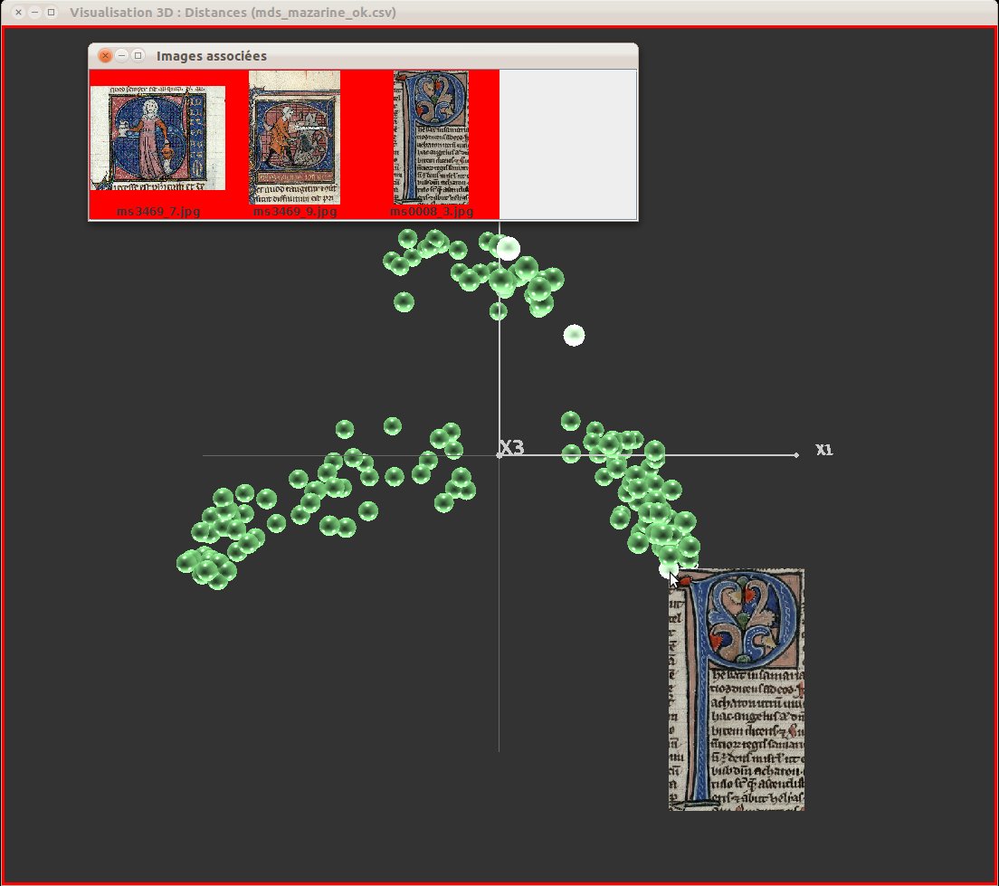
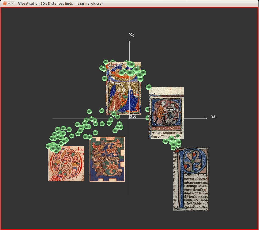
Depending on user’s options (see section 7.7), image static display will occur either in the 3D view or in a specific window. If option “Draw pictures out-of 3D” is checked, then a specific window is use (see fig. 7); otherwise they are directly displayed in the 3D view (see fig. 8).
We can notice, in figure 7, that the objected linked to the pictures have been lected (red background in the picture window, and highlighted color in the 3D view). We can also notice that one image is currently dynamically displayed in the 3D view.
The default option consists in displaying images out-of the 3D view, in a spcific window.
If several images are available for a single object, the user can decide to display them simultaneously using a set of 3D scenes. To be more precise, the user can define a specific image attribute for each of her 3D scenes.
The default configuration consists in using a single image attribute for all of the 3D scenes. If several additional attributes are available, that correspond to the name of picture files, and if the user wishes to view a least two of them simultaneously, the way this can be achieved with Explorer3D consists in creating several 3D scenes, possibly using the same projection, and then associating a specific image attribute to each of these scenes. For this purpose, the user must first activate the view a specific image attribute will be associated with, then check the “Specific A.D.” box in the “Additional attributes” sub-window, and last choose the specific picture attribute. Any scene for which the “Specific A.D.” box has not been checked will use the global image attribute, if any has been defined. Conversely, several scenes can use a specific image attribute.
Multiple picture sources can exist, for instance in the case multisource data, each of this source bringing its own set of images, or more generally in the case images are just a side information of the object studied and not the sources of features.
By default, colors are associated with classes, which means that setting a class attribute implies that the same attribute is automatically set as the color one.
Nevertheless, it is possible to choose a color attribute directly, and thus to dissociate it from the role of class attribute. This also allows gradient colouring (see fig. 9). Gradient colouring is automatically used if the color attribute is of numerical type. Note : Explorer3D does by default consider that additional atributes are of symbolic type. For an additional attribute to be considered numerical, it must be explicitely declared as, in the source file, its name being suffixed with “.N”.
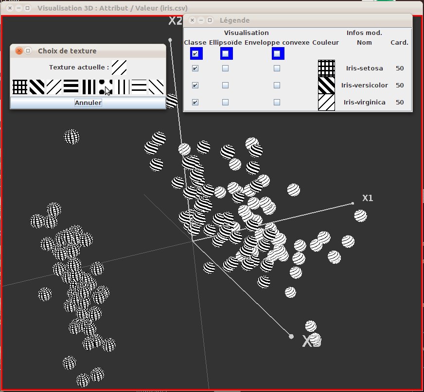
Colours can be replaced with black and white textures. The use of textures is activated by checking the “Texture” box in the “Additional attributes” subwindow. There are currently ab. ten textures available.
The user can change the texture associated with a set of objects by clicking on it in the legend window.
Textures are also displayed on ellipsoids and convex envelopes if these laters are displayed.
Colours remain displayed, in the current release, to highlight selected objects (a selected object will be coloured, even if textures are active; it be become textured again if deselected).
Figure 10 illustrates the use of textures. We can see that the user is currently changing the texture associated with the third group (iris-virginica).
Using a 3-button mouse is recommended. Many tasks can be achieved throught he mouse: selecting objects, displaying information, etc.
Pressing the mouse buttons on the background (i.e. with no object under the mouse pointer), the user obtains the following behaviours:
Right clicking in the 3D scene opens a popup menu, form which various actions can be achieved. When opening the menu while the mouse points on a projected objects, the following ations are proposed:
If the menu is poped up while no object is pointed, only global actions are proposed (global show / hide actions and planar selection).
a uniform selection mecanism has been implemented. There exist several ways to get a object selected: from the 3D scene, from the separated image windows, etc.
When an object gets selected in one of these views, in is also displayed as selected in the other ones. For instance, when an object gets selected in the 3D scene, it gets highlighted in this scene, but the corresponding picture (if displayed) does also get displayed on a red background.
Several objects can be selected at once. Choosing the planar selection in the popup menu allow the user to draw a rectangle in the 3D view (clicking on the background a first time to set the upper left angle, and a second time to set the lower right angle of the rectangle, see fig. 11). All the objects within the rectangle get selected (see fig. 12).
This tool, which can be activated through the popup menu, displays a leans in the 3D scene, that magnifies the objects under it. A very interesting side effect comes from the fact that the magnified objects do also get selected. The user can thus see how objects of a given view spread in other viws, if several are displayed. Magnifying parameters (diameter, coefficient) can be adpted in the “Magnifier” sub-window, which is displayed when the “Aspect” perspective is chosen. Figure 13 illustrates the use of the magnifier.
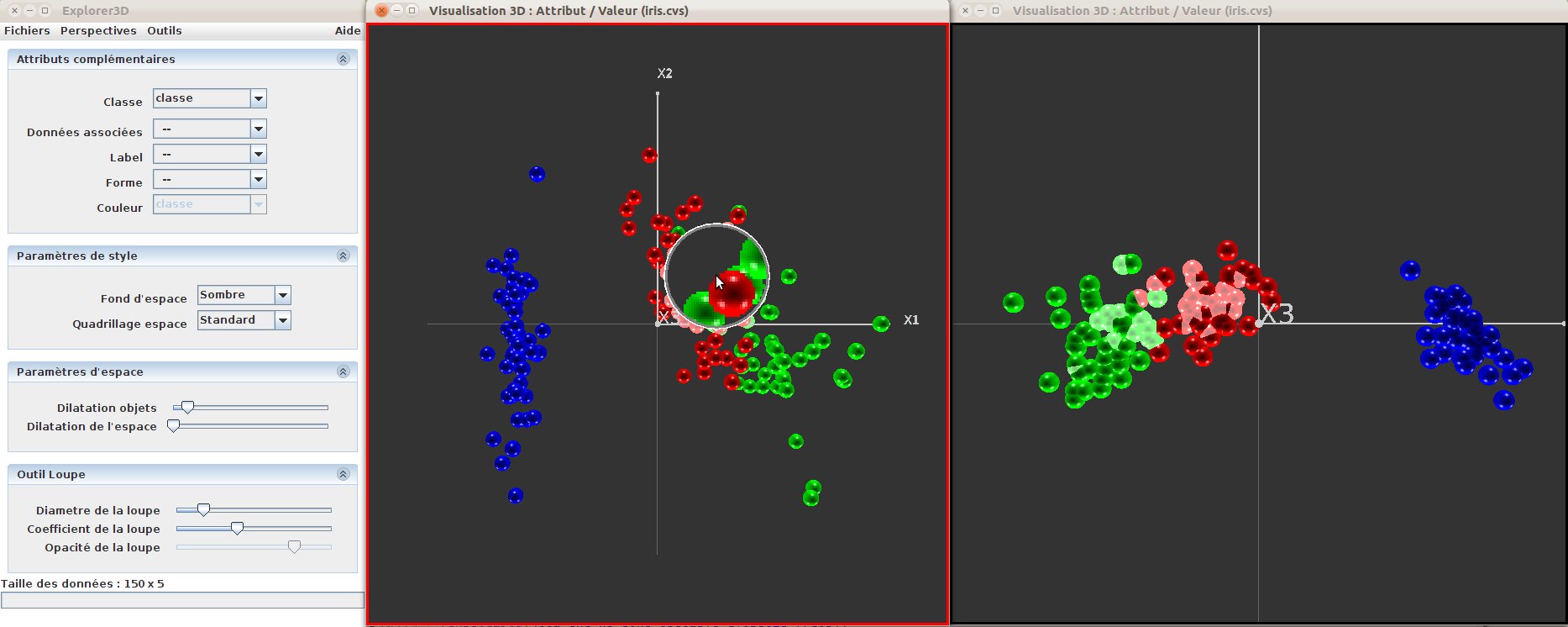
Figure 13: Magnifier. In the left-most scene, selected objects are one that are magnified (to be more precise, the ones that are under the magnifier) in the right-most scene. One can notice the magnifier parameters sub-window, in the control window.
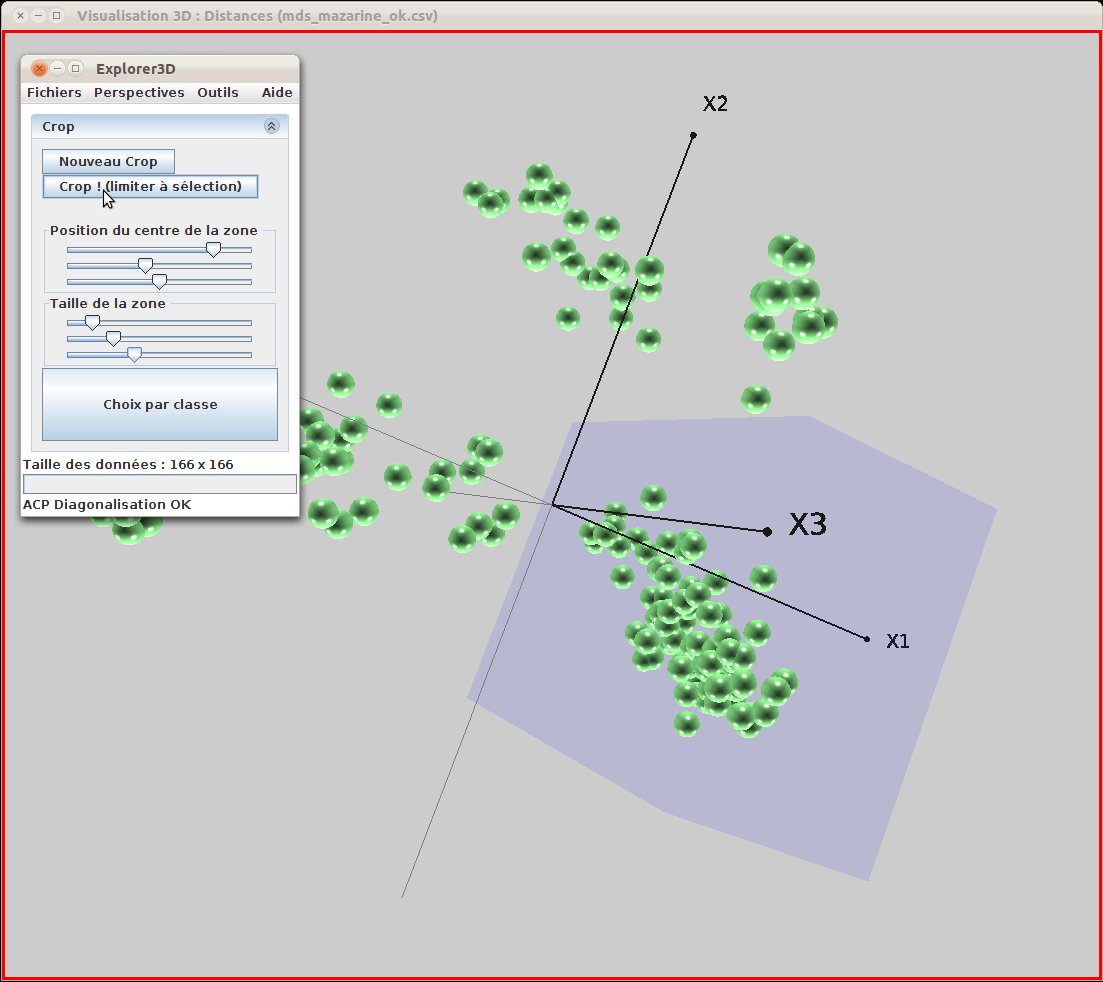
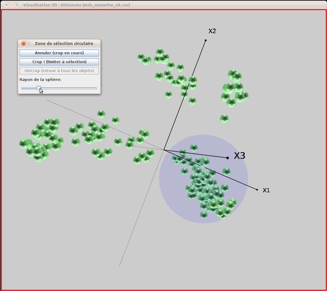
Crop consists in choosing a subset of the objects displayed and then to compute a new projection and scene that fits this subset. The resulting projection can be quite different from the original one.
There are two ways to crop:
When the bow has resized and moved as suited, clicking on “Crop!” causes a new dataset to be produced, that contains the croped object, and a new projection and 3D scene to be computed. Croped view can be croped in turn, and so on.
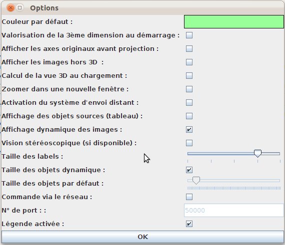
The option window is accessed through the “Tools/options” menu. The current options are:
Depending on the object colouring policy, the legend window displayed will vary. The standard legend window (one colour per object, a finite set of colours) as already been presented in section 6.1. Two others kinds of legend windows are available: the multiclass legend window and the continuous colour attribute legend window.
This legend window is displayed when multiclassification is active. This occurs when the user does manually set a multi-class system (see section 7.2.2) or when a fuzzy classification tool is used (see section 8.3.3). Objects ar coulored according to the class they belong “at most”. Due to Explorer3D current evolutions, additional actions proposed by this legend window are not currently fully functional; nevertheless, the user can visualize the centroïd of each group (appears as a small cross, coloured as the group). Class diffusion through objects can also be observed using convex envelops: by checking “activate convex envelops” and moving the bottom slider, envelop either dilate or shrink to the objects that belong to the class at a higher level than the one indicated by the slider. The “ellipsoïd” column is not currently used.
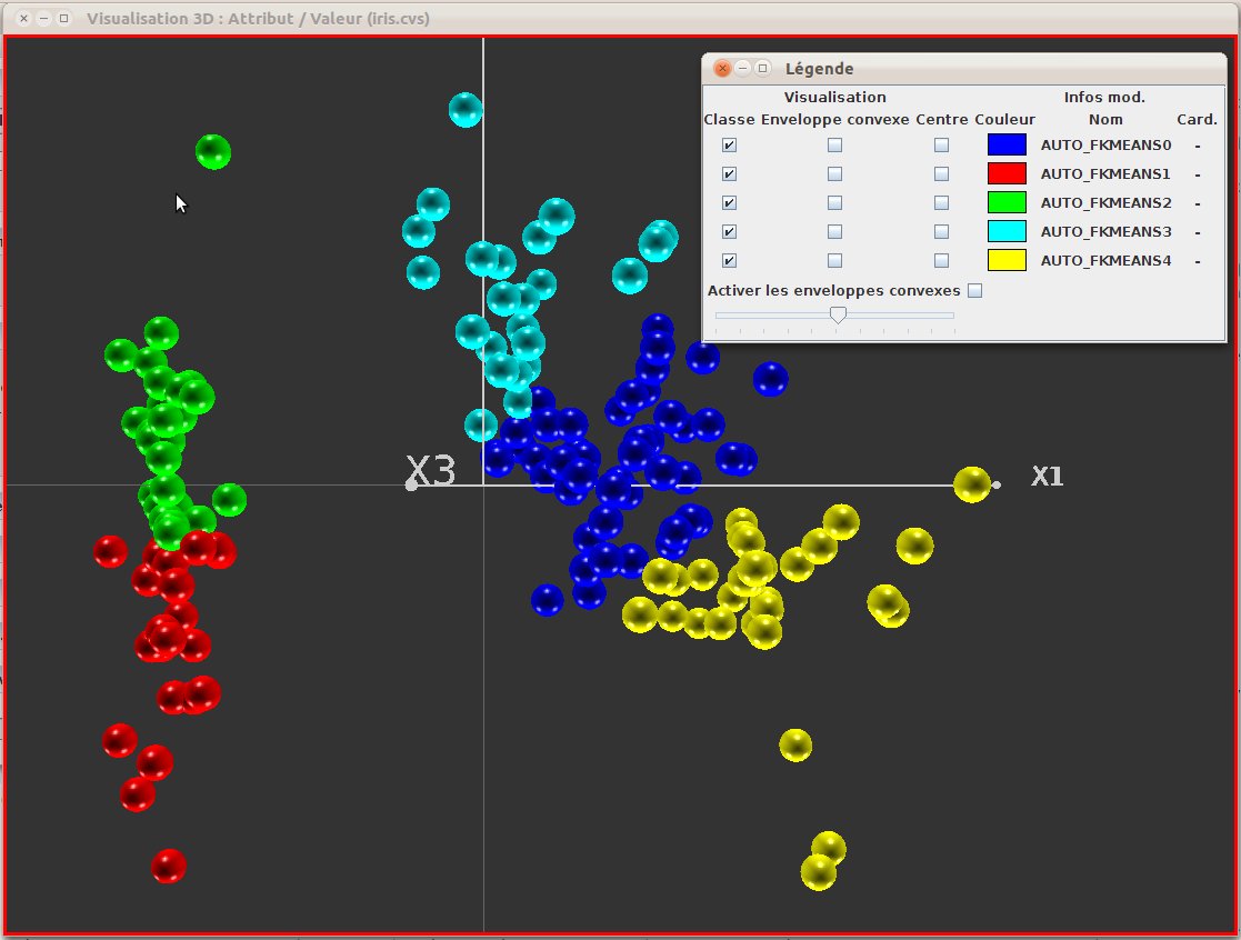
Figure 17: Multiclass legend window. Here we observe a fuzzy kmeans. Each objetct is coloured according to its main class.
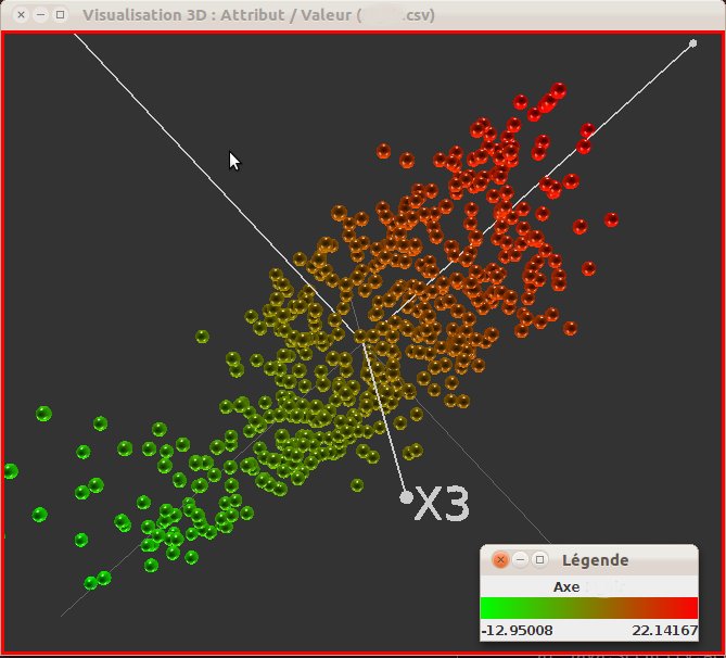
The user can define a colouring that does not rely on a given (set of) class(es), but rather on a single, numerical (floating point) attribute. A colour gradation is then computed to handle any value of the chosen attrifute, from the smallest one to the largest one (see figure 18). Each object gets coloured depending on the attribute value it is associated with. Such a colouring technique is not chosen through the “additional attributes” sub-window. This colouring technique can be activate by three kinds of actions: selection of an explicitely numerical additional attribute as colouring attribute; SVM visualization using colour to materialize the distance of the object to the separating hyperplan (see section 8.6); and materialization of a fourth projection axis by the mean of colouring (see section 7.9). This legend window does only contain the gradation together the min and max values of the attribute.
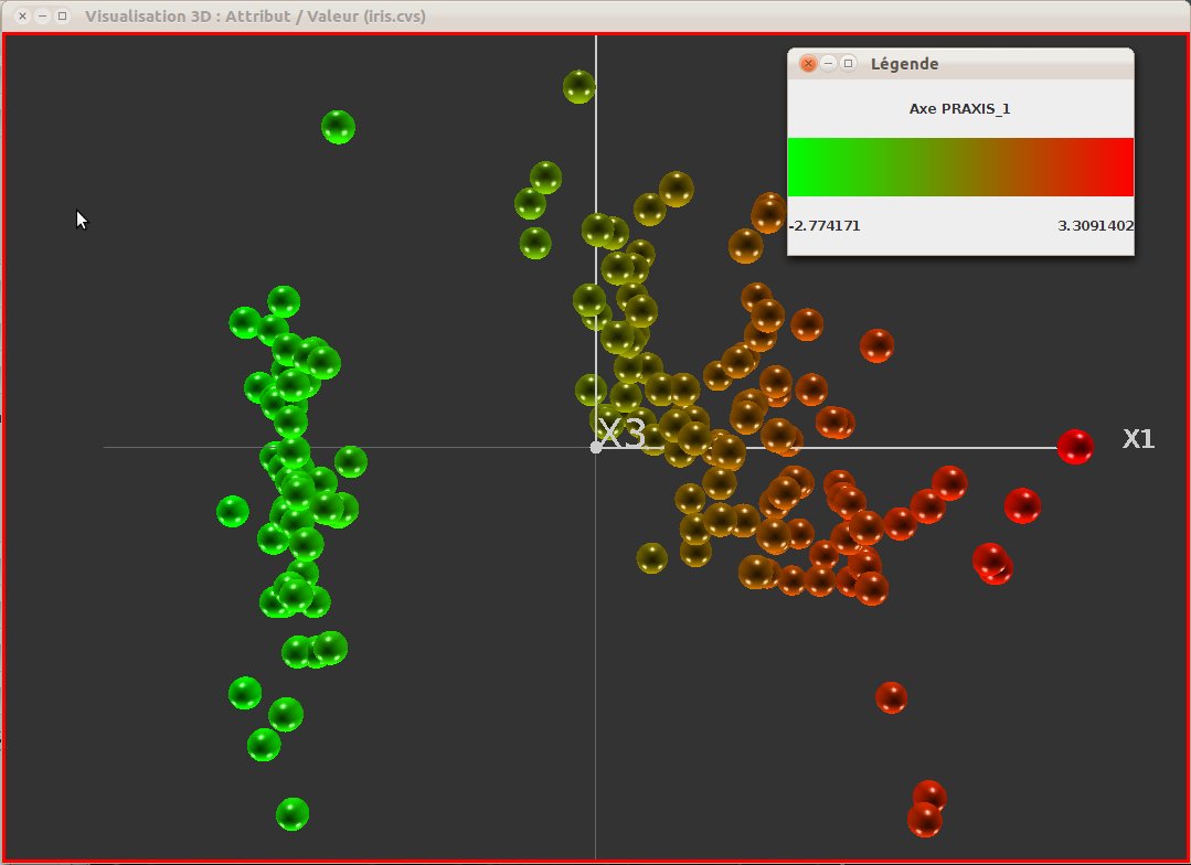
Figure 18: Continuous attribute legend. On can notice that the colouring corresponds to a fourth axis materialization, that in fact is the same as x1.
As introduced in section 7.2.5, colours can be replaced by textures. The legend will allow the user to identify and possibly modify the texture associated with a given group.
The “Projection axes” sub-window allow several actions on the 3D scene. The two first proposed actions are:
This two options do apply to the current scene and to the ones that are computed afterwards.
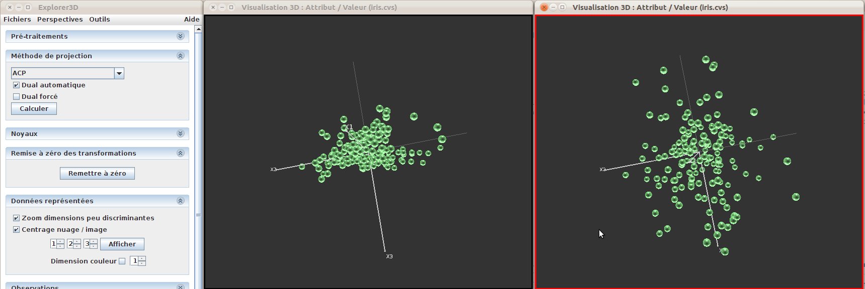
Figure 19: Zoom on less discriminative dimensions et cloud centering. The left-most scene corresponds to a basic PCA projection, the right-most one to the PCA where the two options have been used. The scenes have been rotated so that axes x2 and x3 can be well observed. We can see that objects get more spreaded along x3 in the right-most scene than in the left-most one (this can be also observe, while less important, along x2) and that the object cloud has been translated to the left (centering) compared to the one in the left-most scene.
A third action is available, that alow to choose the projection axes. This functionnality does only make sense when at least three axes are available, that is to say with a “nD->3D” projection, based on feature input data. Nevertheless, the user can always choose at least to invert the dimension-to-axes mapping, or to use the same dimension along several axes. The user can specify the projection dimension used on each axes, in the following order: x1 (breadth), x2 (heigth) and x3 (depth). The scene is only modified once the user clicks on “Draw”. This manually-set projection does not generate a new scene, but rather move objects in the current scene.
The dimensions available are numbered from 1 to n (these are the dimensions computed by the projectin method, not the raw input features). An additional value is given, denoted “X”, which indicates that the corresponding axis is not used. For instance setting x3 to “X” means that objects with all be placed in the x1-x2 plan.
Last, we can choose a projection dimension to colour object (continuous attribute colouring). The coulouring dimensions can be chosen among the projection dimensions computed by the projection method (not among the raw features; this might proposed in a further release). Checking the “Colouring dimension” box, the user activates the continuous attribute colouring, based on the dimension value of each object. Figure 18 illustrates the dimension-based colouring. We can see in this figure that we used the same dimension for colouring as the one used to project objects along x1. Nevertheless, any other available projection dimension might have been used.
This sub-window indicates the amount of original variance that is displayed using the 3 current projection dimensions (figure 20).
a histogramm gives the amount of variance each available projection dimension brings; currently used projection dimensions are drawn red, unused ones are drawn blue.
A pie-chart chart gives the amount of original variance that the current scene offers.
If a class attribute has been selected, then a class purity index is displayed at the bottom of the sub-window (Dunn index).
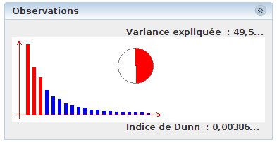
Figure 20: “Observations” sub-window. We can notice that many projection dimensions are available. The three most significant have been chosen for the 3D display (red bars of the histogram), and that they support 49.5 % of the original variance (pie-chart). A class attribute has been selected (the quality of which is displayed, according to the Dunn index).
The user can save the current project, in order to reload it later. The current saving strategy manages data sources, 3D scenes, and the active additional attributes (class, colours, etc.).
To save the current project, choose “Save project” in the “Files” menu. To load a project, choose “Load project”.
Projects are by default saved with the “.e3d” file extension. Technically speaking, they consist of text files using the JSON format.