6 Visualisation interface: an Overview
6.1 Handover
This section consists in a small tutorial on how to use Explorer3D in the context of a PCA.
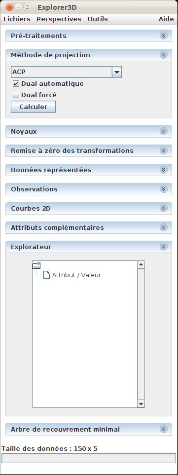
When starting Explorer3D , the main control window opens (cf. fig. 1).
| Figure 1: Explorer3D main control window (at launch time) |
Let us first load the data file. In the menu bar, let use choose “Files / Load local file (new project)”, and pick the iris.csv file.
The main window aspect changes, so that it now offers the functionnalities that are relevant to a feature file (also called the “ND[imensions] → 3D[imensions]” perspective (see fig. 2).
In order to compute a classical PCA, we first check, in the “Pre-treatments” sub-window, that “Center variables” is checked, and that “Reduced variables” is selected in the “Reduction method” list.
Let us then click on “Compute” in the “Projection Method” sub-window.
The 3D view then opens and displays objects using their default shape and colour, that is blue spheres on a dark background (fig. 3).
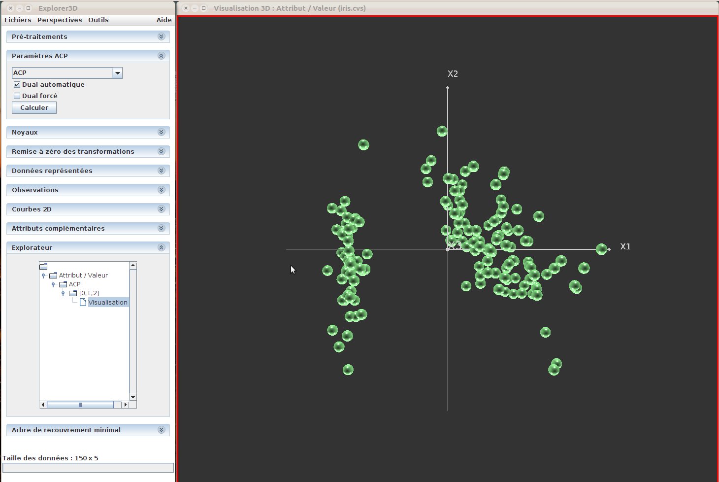
| Figure 3: Default 3D view |
Let us now display an additional visual information, by the mean of object colouring according to their class (each sphere correspond to a given kind of iris, and each kind of iris belongs to one of three varieties).
The class of a given iris (i.e. its variety) is stored in an additional attribute, load together with the features, and named “classe”. Let us display the sub-window “Additional attributes” by clicking on the upper-rigth arrows of this sub-window, and let us choose “classe” in the “Groups” list (which is the only attribute available, let-us ignore “multigroups” for the moment). spheres are then coloured and a legend window pops up (fig. 4).
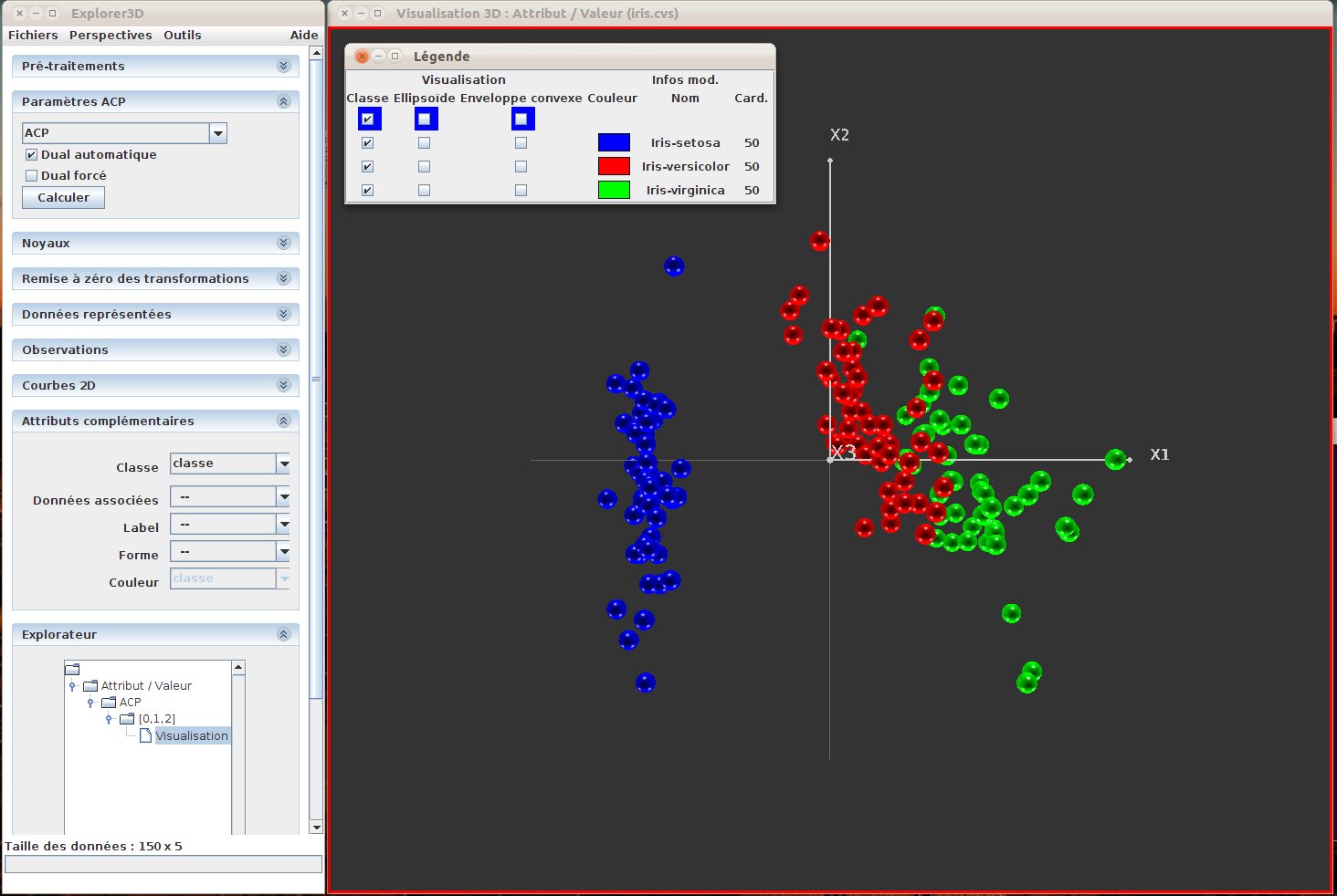
| Figure 4: 3D View with colour and legend |
We can notice the presence of check boxes in the legend window. The “class” check boxes allow to display or hide the objects that belong to a given class.
The “Ellipsoid” checkboxes allow to display an ellipsoid around the corresponding group of objects (i.e. the objects of a given class), that reflects their spreading in space (fig. 5)
(Basically, this ellipsoid is centered on the center of gravity of the group, and its diameters correspond to the variance of the group along its three mains axes, based on the hypothesis of a multinormal distribution).
Figure 5 illustrate a visualisation of objects and the classes ellipsoids.
One must notice that the top-line check boxes (blue background) are shortcuts to check or uncheck the whole column.
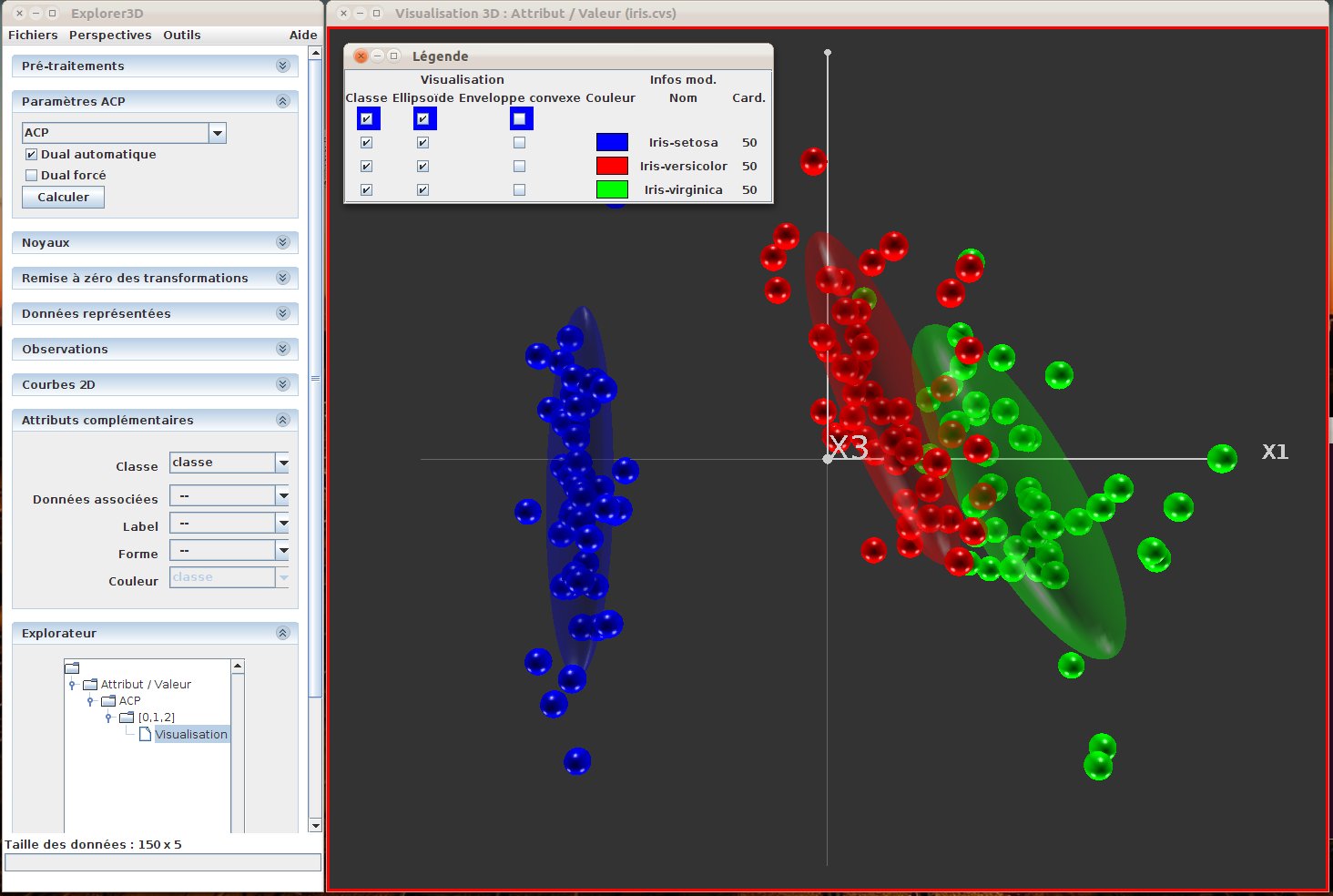
| Figure 5: Groups Ellipsoids |
It is also possible to view the convex envelop of a group. This is done by checking boxes in the “Convex Envelop” column.
Figure 6 illustrates a 3D view where objects have been hiden and only convex envelops are displayed.
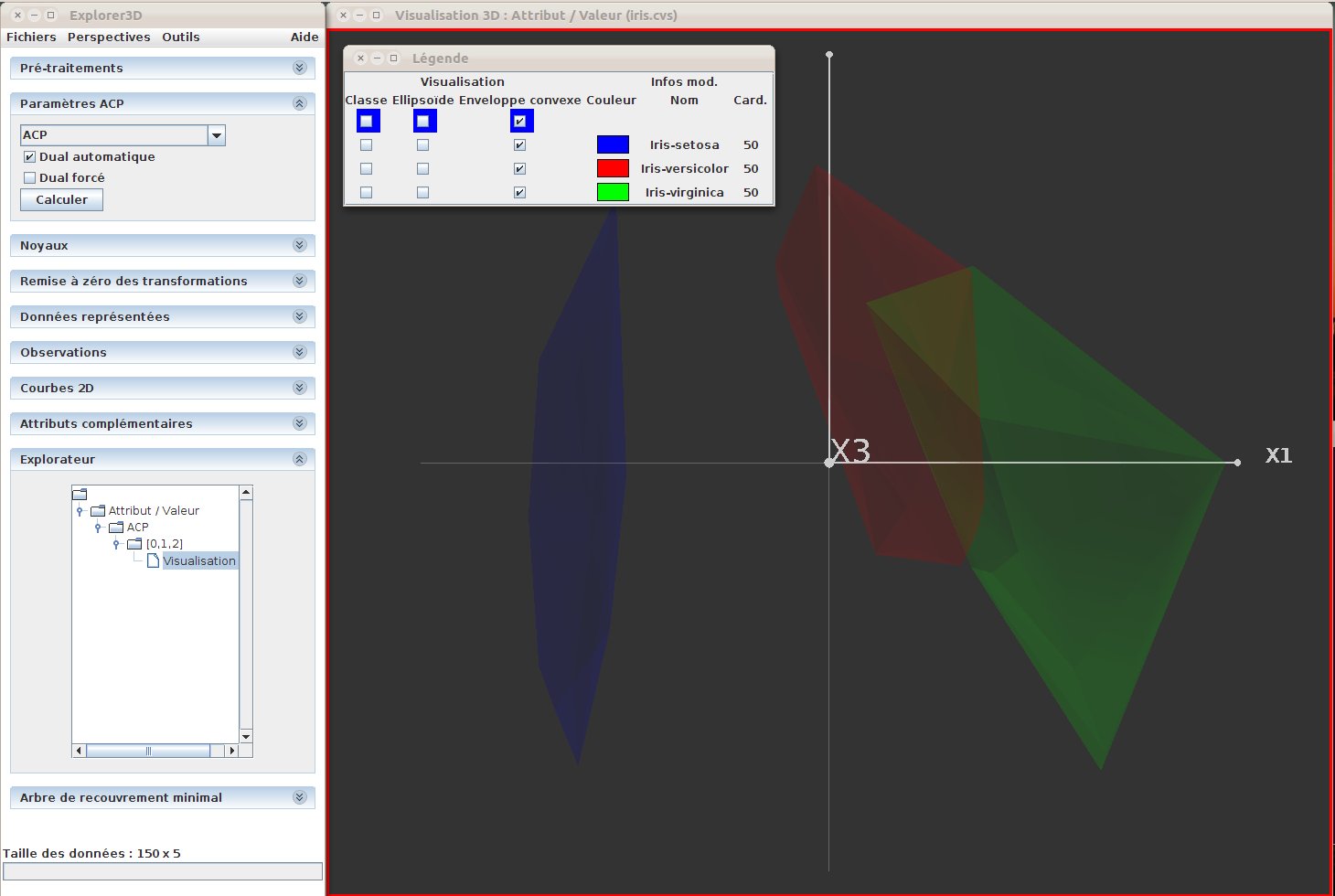
| Figure 6: Convex envelops |
Last, we can interact with the 3D view by using the three mouse buttons (left: rotation; center: zoom; right: translation).
6.2 Control window menus
-
Files: data loading tools
-
Load local file: allow to load the various supported kind of data files. The file content is automatically discovered by Explorer3D . If no standard format is detected, an error message is displayed, and the data import tool is automatically opened.
Let us remind the three kind of data files managed by Explorer3D :
-
Feature files: the file is structured like a table where objects are described by a set of numerical or symbolic features. 3D projection will be computed by the mean of a dimensionnality reduction method (e.g. PCA).
- Distance matrix files: used when the only available data concern the distance or (di)similarity between objects. Projection will be computed by the mean of a MDS.
- Raw 3D coordinates: when we directly get such data, for instance using the output of another software.
- Load online file: this does permit to load a file stored on a distant machine, on a HTTP server. The secondary that opens then allow to set the site URL and then to explorer the web site directories. Supported file formats are the same as for local files.
- Data import tool: This tool allow to the content of a file text and to port it to a Explorer3D -supported file format.
- list of previously loaded files: once a file has been (succesfully) loaded, it gets memorized by Explorer3D and proposed to the user and the bottom of the Files menu.
- Exit: To shut down Explorer3D cleanly.
- Perspectives: This menu leads to some relevant sets of sub-windows with respect to a given kind data file, or to a specific kind of task.
-
ND -> 3D: Perspective that corresponds to features data files (projection from “N” to 3 dimensions).
- Distance -> 3D: Perspective that corresponds to distance matrix files.
- Aspect: Tuning of visual parameters (e.g. background colour, size of objects, etc.).
- Classification: Offers a set of clustering algorithms (e.g. kmeans, gaussian mixtures,...).
- SVM: Offers various SVM visualisation tools, that is to says means to visualize a separating hyperplan between two groups of objects (see section 8.6).
- Tools :
-
Crop: Data cropping based on a 3D box. This consisst in a way to select a subset of objects and compute a new projection that limits to this set of objects and is optimal for that subset (according to the projection criteria). The crop dialog is described in section 7.6.
- Interaction: A tool to modify the projection axes. In this tool one set a list of spatial anomalies and ask for a modified projection that corrects these anomalies. See section 8.4
- Travel thrgough dimensions: A tool to manually set the projection axes by chossing or mixing the axes available. See section 9.1.
- Explore from images: A tool to choose which objects to view in the projection space, together with the associated pictures and nearest neighbors.
See section 8.5.
- Options: To set various options, most of them corresponding to visual elements. See section 7.7.
- Help
-
On-line manual: Opens a browser the browse the on-line version of this manual.
- About Explorer3D : Version facts, mains authors, etc.